First Order ODEs¶

Last time, after a general introduction, we met the general first order ODE:

$$y' = f(t,y).$$

We also examined the very simple, yet interesting such ODE $y'=r y$ and solved it qualitatively (using a slope field) and symbolically (using separation of variables).

Today, we'll generalize those ideas further and explore more challenging examples.

Much of today's material is explored in sections 1.1.3 and 1.3.1 of our text.

The logistic equation¶

Just as the exponential equation $y'=ry$ was a motivating example for us last time, the logistic equation will be a motivating example today:

$$y' = r y (1-y/K).$$

The logistic equation can be interpretted as a growth model, just as the exponential equation can. As we'll see, though, the last $(1-y/K)$ term has the effect of slowing the growth down though as the quantity $y$ approaches the carrying capacity $K$.

Equilibrium solutions¶

Like the exponential equation, the logistic equation is an autonomous equation - not depending explicitly on $t$. When we write an autonomous equation in the form $$y'=f(y),$$ the roots of $f$ form constant or equilibrium solutions of the differential equation.

That is if $y_0$ is a real number with $f(y_0)=0$, then the constant function $y(t) \equiv y_0$ is a solution of the ODE since both sides of $y'=f(y)$ are zero.

Furthermore, if we plot the equilibrium solutions, then they contrain any other solutions.

Logistic equilibrium solutions¶

The logistic equation $y' = r y (1-y/K)$ has two equilibrium solutions, namely

$$ y(t) \equiv 0 \: \text{ and } \: y(t) \equiv K. $$

Let's plot those:

Logistic solutions¶

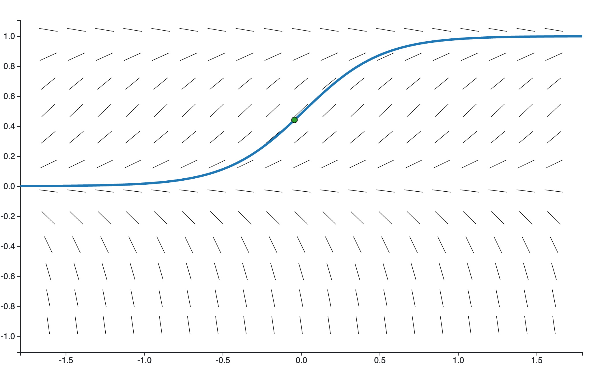
Other solutions to the logistic equation are constrained by the equilibrium solutions. Furthermore, bewtween $0$ and $K$, the right side of the logistic equation

$$y' = r y (1-y/K)$$

is positive (assuming $r$ is positive). Thus, we expect a solution to increase from the bottom equilibrium to the top. Solutions must look something like so:

Logistic slope field¶

We should get a similar sort of picture from a slope field:

The logistic slope field with a solution

Separation of variables¶

Let's apply separation of variables to solve the logistic equation $$ \frac{dy}{dt} = r y (1-y/K) $$ symbolically.

This, is problem #17 from section 1.3.1 of our text.

I guess we'd start with $$ \frac{1}{y(1-y/K)}dy = r\,dt. $$

Separation of variables (cont)¶

The book suggest that we use the partial fractions decomposition

$$ \frac{1}{y(1-K/y)} = \frac{1}{y}+\frac{1}{K-y}, $$

which leads to

$$ \int\left(\frac{1}{y}+\frac{1}{K-y}\right)dy = \int r\,dt $$

$$ \log\left(y\right) - \log\left(K-y\right) = r\,t+c_1. $$

Separation of variables (cont 2)¶

Combining the logarithms in that last equation yields

$$ \log\left(\frac{y}{K-y}\right) = r\,t+c_1, $$

which allows us to apply the exponential to both sides to get

$$ \frac{y}{K-y} = e^{r\,t+c_1} = c e^{r\,t}. $$

Note that we've pulled the old $e^{a+c_1} = e^ae^{c_1} = e^ac$ trick.

Separation of variables (cont 3)¶

Now, we can solve that last equation for $y$ to get

$$ y = \frac{K\,c\,e^{r\,t}}{1+c\,e^{r\,t}} = \frac{K}{1+\frac{1}{c}e^{-r\,t}}. $$

That is our solution:

$$y(t) = \frac{K}{1+\frac{1}{c}e^{-r\,t}}.$$

Interpretation¶

Given our solution,

$$y(t) = \frac{K}{1+\frac{1}{c}e^{-r\,t}},$$

It's not hard to see that

$$\lim_{t\to -\infty}y(t) = 0 \: \text{ and } \: \lim_{t\to\infty}y(t)=K$$

and that $y$ increases from $0$ to $K$ as $t$ ranges from $-\infty$ to $\infty$.

That agrees with our qualitative analysis!

An IVP¶

In order to plot a specific solution, we'll need values for the parameters $r$ and $K$, as well as an initial condition. Let's assume that

$$K=100, \: r=3, \text{ and } y(0)=4.$$

Thus, our solution becomes

$$y(t) = \frac{100}{1+\frac{1}{c}e^{-3\,t}}.$$

An IVP (cont)¶

To find $c$ in

$$y(t) = \frac{100}{1+\frac{1}{c}e^{-3\,t}},$$

we use the initial condition $y(0)=4$ to get

$$4 = \frac{100}{1+\frac{1}{c}}.$$

We solve this to get $c=1/24$ so that

$$y(t) = \frac{100}{1+24e^{-3\,t}}.$$

Here's how to plot that solution in Python:

import matplotlib.pyplot as plt
import numpy as np
def y(t): return 100/(1+24*np.exp(-3*t))
ts = np.linspace(-1,5)
ys =  y(ts)
plt.plot(ts,ys);

Slope fields for autonomous equations¶

The logistic equation is somewhat indicative of the way that the general autonomous equation $y'=f(y)$ works.

We first find the equilibrium solutions; then, assuming that $f$ is continous, the slopes don't change sign between the equilibria.

Then, it's easy to sketch the solutions.

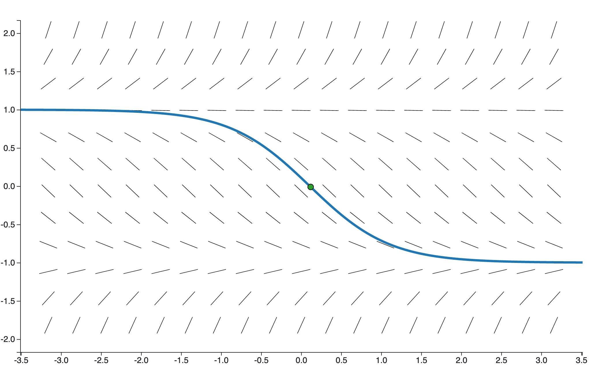
Example¶

For example, here's the slope field for $y'=y^2-1$, together with a solution between the two equilibria of $\pm 1$, which must be decreasing:

Slope field of y'=y^2-1, together with a decreasing solution

Finally...¶

How about I do one by hand?