Subsection1.1.3Newton's method in the complex domain

Let's move now to the complex domain, where even crazier things can happen. To understand this stuff, of course, you'll need a basic understanding of complex numbers but it's really not a daunting amount of information. You'll need to know that a complex number \(z\) has the form

\begin{equation*} z = x+iy, \end{equation*}

where \(x\) and \(y\) are real numbers (the real and imaginary parts of \(z\)) and \(i\) is the imaginary unit (thus \(i^2=-1\)). You'll also need to know (or accept) that you can do arithmetic with complex numbers and plot them in a plane, called the complex plane. We'll discuss complex variables in a more detail when we jump into complex dynamics more completely.

Subsubsection1.1.3.1Cayley's question

In the 1870s, the prolific British mathematician Arthur Cayley (whose name is all over abstract algebra) posed the following interesting question: Given a Suppose that \(p\) is a complex polynomial and \(z_0\) is an initial seed that we might use for Newton's method. Generally, \(p\) will have several roots scattered throughout the complex plane. Is it possible to tell to which of those roots (if any) Newton's method will converge to when we start at \(z_0\text{?}\)

Generally, the closer an initial seed is to a root, the more likely that seed will lead to a sequence that converges to the root. It might be reasonable to guess that the process always converges to the root that is closest to the initial seed. Cayley proved that this is true for quadratic functions but was commented that the general question is much more difficult for cubics. With the power of the computer, there is a very colorful way to explore the question

Algorithm1.1.9Coloring basins of attraction for Newton's method

Given: A function \(f:\mathbb C \to \mathbb C\text{.}\)
Choose a rectangle \(R\) in the complex plane with sides parallel to the real and imaginary axes.
- The points in \(R\) represent potential initial seeds when applying Newton's method to \(f\text{.}\)
Discretize the rectangle into points of the form \begin{equation*} z_{0,jk} = (a+j\Delta x) + (b + k\Delta y)k. \end{equation*}
For each point \(z_{0,jk}\) perform Newton's iteration to generate a sequence \((z_{n,jk})_n\) until one of two things happen:
- \(|f(z_{n,jk})| < \varepsilon\text{,}\) where \(\varepsilon\) is some pre-specified small number. We assume that the process has converged to a root; color the initial seed \(z_{0,jk}\) according to which root the process converged to and shade the initial seed according to how many iterates this process took.
- The iteration count exceeds some pre-specified bailout; we color the initial seed \(z_{0,jk}\) black.

Let's take a look at a simple, quadratic example.

Example1.1.10

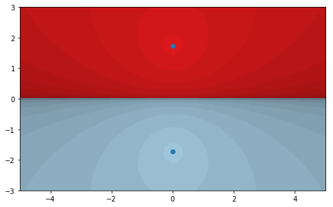
Let \(p(z)=z^2+3\text{.}\) We already played with this function in the real case back in Example 5 and the computer indicated that there might be chaos on the real line. When we allow complex inputs, though, there are two roots - one at \(\sqrt{3}i\) (above the real axis) and one at \(-\sqrt{3}i\) (below the real axis). If the process always converges to the root that is closest to the initial seed, then seeds in the upper half plane should converge to \(\sqrt{3}i\) while seeds in the lower half plane should converge to \(-\sqrt{3}i\text{.}\) We don't have the tools to prove this yet, but we can investigate with Algorithm 9. The result is shown in Figure 11.

Figure1.1.11Attractive basins for \(f(z)=z^2+3\)

Now, let's take a look at a classic, cubic example.

Example1.1.12

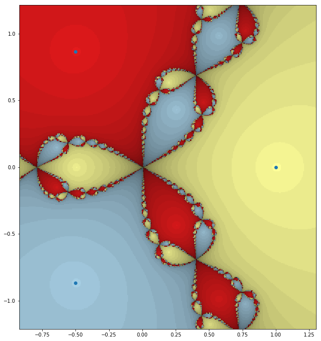
Let \(p(z)=z^3 - 1\text{.}\) As a complex, cubic polynomial, we expect \(p\) to have three roots. It's easy to see that \(z=1\) is a root. This means that \(z-1\) is a factor, which makes it easier to find that

\begin{equation*} p(z) = (z-1)(z^2+z+1). \end{equation*}

We can then apply the quadratic formula to find that the other two roots are

\begin{equation*} \frac{-1\pm\sqrt{-3}}{2} = -\frac{1}{2}\pm\frac{\sqrt{3}}{2}i. \end{equation*}

Note that all three roots can be clearly seen in Figure 13, which shows the result of Algorithm 9.

Figure1.1.13Attractive basins for \(f(z)=z^2+3\)

Figure 13 is just an incredible picture. We can clearly see the three roots of \(p\) and, indeed, if we start close enough to a root we do converge to that root. The boundary between the basins seems to be incredibly complicated, though.

As a final example, let's take a look at the complex cosine.

Example1.1.14

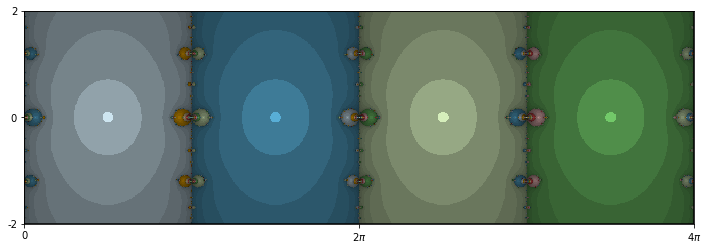
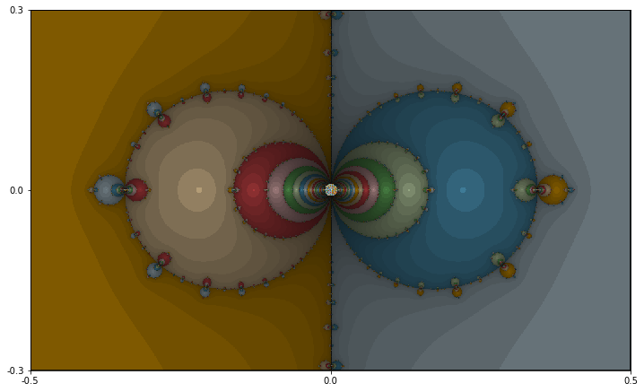
Let \(f(z)=\cos(z)\text{.}\) Of course, we played with the real cosine back in Example 7. There, we saw that in any tiny interval containing zero, an initial seed might converge to any of infinitely many roots. In the complex case, the basins of attraction are shown in Figure 15, and a zoom is shown in Figure 16.

Figure1.1.15Attractive basins for the cosine

Figure1.1.16A zoom into the basins of the cosine

Two more incredible pictures! Note the periodicity in Figure 15. Each root seems to have its own column of attraction. The boundaries between the basins are again very complicated. In the zoom of Figure 16, t looks like there's an infinite sequence of circles collapsing on either side of the origin. This agrees with our observations in the real case of Example 7.

Generating pictures for the Newton's method is great fun. There is an online tool that allows you to generate the basins of attraction for an (almost) arbitrary polynomial here:

https://marksmath.org/visualization/complex_newton/.